pyCactus Demo
This notebook demonstrates the core functionality of the pyCactus
post-processing module.
Author: Phillip Chiu
In [1]:
# enable autoreload
%load_ext autoreload
%autoreload 2

# set up plotting backend
# %matplotlib nbagg
%matplotlib inline

import matplotlib
import matplotlib.pyplot as plt

# matplotlib.rcParams['figure.figsize'] = (14.0, 10.5)  # large figures
matplotlib.rcParams['figure.figsize'] = (8, 6)         # medium figures
matplotlib.rcParams.update({'font.size': 14})          # label size

# set up paths
import os
import sys

nb_root_dir = os.path.expanduser('~/Notebooks/')      # notebook root dir
nb_dir_name = 'demo1'                                 # notebook work dir name
nb_dir = os.path.abspath(os.path.join(nb_root_dir,
                                      nb_dir_name))   # notebook work dir

# create notebook dir if it doesn't exist
if not os.path.exists(nb_dir):
    os.makedirs(nb_dir)

sys.path.append(nb_dir) # append notebook work dir to pythonpath
os.chdir(nb_dir)        # change path to notebook work dir

# import commonly-used modules
import math
import numpy as np
import pandas as pd
import time as pytime

# apply style (from external notebook)
%run '~/Notebooks/style.ipynb'
clean()
Out[1]:
Add the path to pyCactus and import.
In [2]:
sys.path.append(nb_dir + '/CACTUS-tools/')
import pyCactus
Creating a CactusRun instance
The CactusRun reads and stores information about a single run. The
path to the data files is specified when initializing the CactusRun
instance. It can be instantiated as follows:
In [3]:
case_name  = 'NREL-5MW'
run_dir    = os.path.join(nb_dir,'NREL-5MW-CACTUS')
In [4]:
tic = pytime.time()
geom_fname = 'NREL-5MW.geom'
run = pyCactus.CactusRun(run_dir, case_name,
                         geom_fname=geom_fname,
                         wakeelem_fnames_pattern='*WakeData_*.csv',
                         field_fnames_pattern='*WakeDefData_*.csv')
print 'Time to instantiante CactusRun class: %2.2f s' % (pytime.time() - tic)
Read input namelist in 0.01 s
Read geometry file in 0.01 s
Read parameter data in 0.00 s
Read revolution-averaged data in 0.00 s
Read blade element data in 0.06 s
Read time data in 0.01 s
Read 20 wake element data headers in 0.00 s
Read 20 wake element data headers in 0.00 s
Read grid dimensions in 0.05 s
Read 6 probe data file headers in 0.00 s

Success: Loaded case `NREL-5MW` from path `/home/phil/Notebooks/demo1/NREL-5MW-CACTUS`

Time to instantiante CactusRun class: 0.17 s
On instantiation, the CactusRun class loads the geometry file along
with the time data, blade element data, and revolution-averaged data. It
also parses the first line of each of the wake grid and wake node
.csv files to determine the output times.
The time, element, and revolution data are stored as Pandas dataframes. In order to reduce both memory usage and the time for class instantiation, data is only read from wake element and field data files (which may be very large) when needed.
Geometry data
The geometry data can be accessed easily by calling the
CactusRun.geom attribute, which is an instance of the CactusGeom
class.
The geometry data is stored in the globalvars, blades, and
struts attributes.
In [5]:
run.geom.globalvars
Out[5]:
{'NBlade': [3],
 'NStrut': [0],
 'RefAR': array([ 3.14159]),
 'RefR': array([ 206.693]),
 'RotN': array([ 1.,  0.,  0.]),
 'RotP': array([ 0.,  0.,  0.]),
 'Type': ' HAWT'}
The blades and struts are lists of variable dictionaries,
enumerated by blade number and strut number.
In [6]:
blade_num = 0
run.geom.blades[blade_num].keys()
Out[6]:
['ECtoR',
 'nEz',
 'nEx',
 'nEy',
 'tz',
 'PEy',
 'PEz',
 'ty',
 'QCz',
 'QCy',
 'QCx',
 'iSect',
 'EAreaR',
 'NElem',
 'dr_over_R',
 'r_over_R_elem',
 'FlipN',
 'PEx',
 'CtoR',
 'tx',
 'Blade 1',
 'sEz',
 'sEy',
 'sEx',
 'tEx',
 'tEy',
 'tEz']
Accessing time, revolution-averaged, and blade element data
Time, blade element, and revolution data can be accessed using the appropriate variables names:
CactusRun.time_dataCactusRun.elem_dataCactusRun.rev_data
Each returns a Pandas dataframe whose column names are shown below.
Time data
The column names for the time data are shown below.
In [7]:
run.time_data.columns
Out[7]:
Index([u'Normalized Time (-)', u'Theta (rad)', u'Rev', u'Torque Coeff. (-)',
       u'Power Coeff. (-)', u'Fx Coeff. (-)', u'Fy Coeff. (-)',
       u'Fz Coeff. (-)', u'Blade Fx Coeff. (-)', u'Blade Fy Coeff. (-)',
       u'Blade Fz Coeff. (-)', u'Blade Torque Coeff. (-)',
       u'Blade Fx Coeff. (-).1', u'Blade Fy Coeff. (-).1',
       u'Blade Fz Coeff. (-).1', u'Blade Torque Coeff. (-).1',
       u'Blade Fx Coeff. (-).2', u'Blade Fy Coeff. (-).2',
       u'Blade Fz Coeff. (-).2', u'Blade Torque Coeff. (-).2'],
      dtype='object')
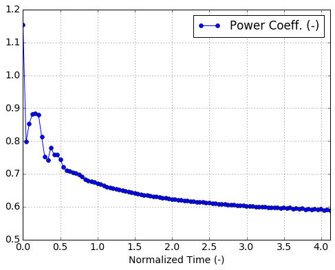
It is easy to plot this data. Here we use the built-in plotting feature of the Pandas dataframe, but this could also be done with NumPy.
In [8]:
plt.figure()
run.time_data.plot(x='Normalized Time (-)',y='Power Coeff. (-)',
                   marker='o')
plt.grid(True)
<matplotlib.figure.Figure at 0x7fe0d02ae0d0>
Revolution-averaged data
The column names for the revolution-averaged data are shown below.
In [9]:
run.rev_data.columns
Out[9]:
Index([u'Rev', u'Power Coeff. (-)', u'Tip Power Coeff. (-)',
       u'Torque Coeff. (-)', u'Fx Coeff. (-)', u'Fy Coeff. (-)',
       u'Fz Coeff. (-)', u'Power (kW)', u'Torque (ft-lbs)'],
      dtype='object')
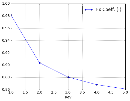
As with the time data, this can be easily plotted.
In [10]:
plt.figure()
run.rev_data.plot(x='Rev',y='Fx Coeff. (-)',
                   marker='o')
plt.grid(True)
<matplotlib.figure.Figure at 0x7fe0ae2b6b50>
Blade element data
The column names for the blade element data are shown below.
In [11]:
run.bladeelem_data.data.columns
Out[11]:
Index([u'Normalized Time (-)', u'Theta (rad)', u'Blade', u'Element', u'Rev',
       u'x/R (-)', u'y/R (-)', u'z/R (-)', u'AOA25 (deg)', u'AOA50 (deg)',
       u'AOA75 (deg)', u'AdotNorm (-)', u'Re (-)', u'Mach (-)', u'Ur (-)',
       u'IndU (-)', u'IndV (-)', u'IndW (-)', u'GB (?)', u'CL (-)', u'CD (-)',
       u'CM25 (-)', u'CLCirc (-)', u'CN (-)', u'CT (-)', u'Fx (-)', u'Fy (-)',
       u'Fz (-)', u'te (-)'],
      dtype='object')
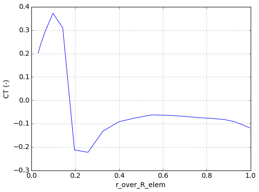
This data can also be plotted easily. We can extract the blade data at a
particular time index by calling
CactusRun.blade_data_at_time_index().
For horizontal axis wind turbines, it is often desirable to plot a blade
quantity against the distance from the rotation axis. This is
demonstrated here using data from the CactusRun.geom instance.
In [12]:
blade_num = 0

# get the blade data at the final time index
time, dfs_blade = run.bladeelem_data.data_at_time_index(time_index=-1)

plt.figure()
plt.plot(run.geom.blades[blade_num]['r_over_R_elem'],
         dfs_blade[blade_num]['CT (-)'])
plt.grid(True)
plt.xlabel('r_over_R_elem')
plt.ylabel('CT (-)')
plt.show()
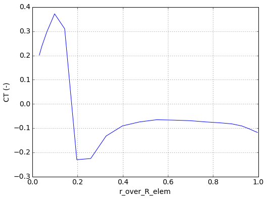
The blade data can also be time-averaged over specified timesteps. In the following example, we average over the last 5 timesteps.
In [13]:
timesteps = range(-5,0)
CT_averaged = run.bladeelem_data.data_time_average('CT (-)', timesteps, 1)

timesteps
Out[13]:
[-5, -4, -3, -2, -1]
In [14]:
plt.figure()
plt.plot(run.geom.blades[blade_num]['r_over_R_elem'],
         CT_averaged)
plt.grid(True)
plt.xlabel('r_over_R_elem')
plt.ylabel('CT (-)')
plt.show()
Accessing wake element and field data
Due to their potentially large file sizes, wake element and field data are accessed differently than the above data – the entire data file is never loaded into memory.
Wake element data
Viewing times
The times at which we have wake element data can be easily viewed.
In [15]:
run.wakeelems.num_times
Out[15]:
20
In [16]:
run.wakeelems.times
Out[16]:
array([ 0.       ,  0.2080525,  0.416105 ,  0.6241575,  0.83221  ,
        1.040262 ,  1.248315 ,  1.456367 ,  1.66442  ,  1.872472 ,
        2.080525 ,  2.288577 ,  2.49663  ,  2.704682 ,  2.912735 ,
        3.120787 ,  3.32884  ,  3.536892 ,  3.744945 ,  3.952997 ])
Extracting data to NumPy arrays
A dataframe containing data at a particular timestep can be extracted
using the method CactusWakeElem.get_df_inst(). This returns a
dictionary containing variables names and their values as NumPy arrays.
In [17]:
# Get dataframe for a specific time
ti = 5
wake_df_inst = run.wakeelems.get_df_inst(time=run.wakeelems.times[ti])
wake_df_inst.head()

# extract variables
wakeelemdata, has_node_ids = run.wakeelems.wakedata_from_df(wake_df_inst)
In [18]:
wakeelemdata.keys()
Out[18]:
['node_ids', 'elems', 'u', 'w', 'v', 'y', 'x', 'z']
The second return is a flag which indicates whether the wake element
data files have a node_id column. (For compatibility with data
generated by versions of CACTUS).
In [19]:
has_node_ids
Out[19]:
True
Writing to VTK
The wake element data can be written to a VTK file to facilitate
post-processing with ParaView or other tools. To do this, we can use the
CactusWakeElems.write_vtk_series() method. This writes a series of
VTK files, and a .pvd collection file which can be read into
ParaView directly as a time series.
In [20]:
wakeelem_output_path = os.path.join(nb_dir,'vtk')
run.wakeelems.write_vtk_series(wakeelem_output_path,
                               'wakenode_name',
                               print_status=False)
Out[20]:
(['/home/phil/Notebooks/demo1/vtk/wakenode_name_0.vtu',
  '/home/phil/Notebooks/demo1/vtk/wakenode_name_1.vtu',
  '/home/phil/Notebooks/demo1/vtk/wakenode_name_2.vtu',
  '/home/phil/Notebooks/demo1/vtk/wakenode_name_3.vtu',
  '/home/phil/Notebooks/demo1/vtk/wakenode_name_4.vtu',
  '/home/phil/Notebooks/demo1/vtk/wakenode_name_5.vtu',
  '/home/phil/Notebooks/demo1/vtk/wakenode_name_6.vtu',
  '/home/phil/Notebooks/demo1/vtk/wakenode_name_7.vtu',
  '/home/phil/Notebooks/demo1/vtk/wakenode_name_8.vtu',
  '/home/phil/Notebooks/demo1/vtk/wakenode_name_9.vtu',
  '/home/phil/Notebooks/demo1/vtk/wakenode_name_10.vtu',
  '/home/phil/Notebooks/demo1/vtk/wakenode_name_11.vtu',
  '/home/phil/Notebooks/demo1/vtk/wakenode_name_12.vtu',
  '/home/phil/Notebooks/demo1/vtk/wakenode_name_13.vtu',
  '/home/phil/Notebooks/demo1/vtk/wakenode_name_14.vtu',
  '/home/phil/Notebooks/demo1/vtk/wakenode_name_15.vtu',
  '/home/phil/Notebooks/demo1/vtk/wakenode_name_16.vtu',
  '/home/phil/Notebooks/demo1/vtk/wakenode_name_17.vtu',
  '/home/phil/Notebooks/demo1/vtk/wakenode_name_18.vtu',
  '/home/phil/Notebooks/demo1/vtk/wakenode_name_19.vtu'],
 '/home/phil/Notebooks/demo1/vtk/wakenode_name.pvd')
Field data
Viewing times
In [21]:
run.wakeelems.num_times
Out[21]:
20
In [22]:
run.field.times
Out[22]:
array([ 0.       ,  0.2080525,  0.416105 ,  0.6241575,  0.83221  ,
        1.040262 ,  1.248315 ,  1.456367 ,  1.66442  ,  1.872472 ,
        2.080525 ,  2.288577 ,  2.49663  ,  2.704682 ,  2.912735 ,
        3.120787 ,  3.32884  ,  3.536892 ,  3.744945 ,  3.952997 ])
Extracting data to NumPy arrays
A dataframe containing data at a particular timestep can be extracted
using the method CactusField.get_df_inst(). This returns a
dictionary containing variables names and their values as NumPy arrays.
In [23]:
# Get dataframe for a specific time
ti = 5
field_df_inst = run.field.get_df_inst(time=run.wakeelems.times[ti])
field_df_inst.head()

# extract variables
fielddata, fielddims = run.field.fielddata_from_df(field_df_inst)
In [24]:
fielddata.keys()
Out[24]:
['Ufs', 'Wfs', 'U', 'W', 'V', 'Y', 'X', 'Z', 'Vfs']
The second return is a dictionary of the field dimensions.
In [25]:
fielddims
Out[25]:
{'dx': 0.0,
 'dy': 0.040000000000000001,
 'dz': 0.040000000000000001,
 'nx': 1,
 'ny': 100,
 'nz': 100,
 'xlim': [0.0, 0.0],
 'ylim': [-2.0, 2.0],
 'zlim': [-2.0, 2.0]}
The dimensions of the returned arrays match the grid dimensions.
In [26]:
fielddata['U'].shape
Out[26]:
(100, 100, 1)
Time series at a specific location on the Cartesian grid
Data at a specific location can be extracted. This operation may take some time, since it loops through all the data files.
In [27]:
# enter a list of point coordinates
point_list = [(0.0, 0.5, 0.5),
              (1.0, 0.0, 0.0)]

tic = pytime.time()
timeseries_dict, nearest_points = run.field.pointdata_time_series(point_list, ti_start=0, ti_end=-1)
print 'Time to produce series: %2.2f s' % (pytime.time() - tic)

print nearest_points
Time to produce series: 0.70 s
[(0.0, 0.50505048, 0.50505048), (0.0, -0.02020202, -0.02020202)]
In [28]:
# extract the data
t   = timeseries_dict['t']
u   = timeseries_dict['u']
v   = timeseries_dict['v']
w   = timeseries_dict['w']
ufs = timeseries_dict['ufs']
vfs = timeseries_dict['vfs']
wfs = timeseries_dict['wfs']
In [29]:
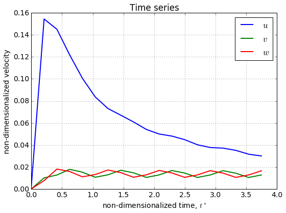
point_id = 1

print t
# plot the data at the point_id'th point
plt.figure()
plt.plot(t, u[point_id,:], label='$u$', lw=2)
plt.plot(t, v[point_id,:], label='$v$', lw=2)
plt.plot(t, w[point_id,:], label='$w$', lw=2)

plt.title('Time series')
plt.xlabel('non-dimensionalized time, $t^*$')
plt.ylabel('non-dimensionalized velocity')
plt.legend(loc='best')

plt.grid(True)
plt.tight_layout()
plt.show()
[ 0.         0.2080525  0.416105   0.6241575  0.83221    1.040262   1.248315
  1.456367   1.66442    1.872472   2.080525   2.288577   2.49663    2.704682
  2.912735   3.120787   3.32884    3.536892   3.744945 ]
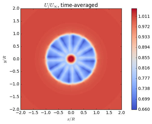
Field averaging
We can time average the field data using the
CactusField.field_time_average() method. This returns a dictionary
containing the averaged data.
In [30]:
tic = pytime.time()

averaged_data = run.field.field_time_average(ti_start=-5,
                                             ti_end=-1)

print 'Time to average fields: %2.2f s' % (pytime.time() - tic)
Time to average fields: 0.19 s
In [31]:
print averaged_data.keys()
['Ufs', 'U', 't', 'W', 'V', 'Y', 'X', 'Z', 'Vfs', 'Wfs']
The t field gives the normalized times which were averaged.
In [32]:
print averaged_data['t']
[ 3.120787 3.32884 3.536892 3.744945]
The averaged data may be plotted.
In [33]:
import matplotlib.cm as cm

# Get the data
X   = averaged_data['X']
Y   = averaged_data['Y']
Z   = averaged_data['Z']
U   = averaged_data['U']
V   = averaged_data['V']
W   = averaged_data['W']
Ufs = averaged_data['Ufs']
Vfs = averaged_data['Vfs']
Wfs = averaged_data['Wfs']

# Reshape to 2D
ny = run.field.grid_dims['ny']
nz = run.field.grid_dims['nz']

X   = np.reshape(X, [ny, nz])
Y   = np.reshape(Y, [ny, nz])
Z   = np.reshape(Z, [ny, nz])
U   = np.reshape(U, [ny, nz])
V   = np.reshape(V, [ny, nz])
W   = np.reshape(W, [ny, nz])
Ufs = np.reshape(Ufs, [ny, nz])
Vfs = np.reshape(Vfs, [ny, nz])
Wfs = np.reshape(Wfs, [ny, nz])

# u
fig = plt.figure()
ax = fig.add_subplot(111)
cax = ax.contourf(Y,Z,U+Ufs,128,cmap=cm.coolwarm)
fig.colorbar(cax)
ax.axis('image')
ax.set_title('$U/U_{\infty}$, time-averaged')
ax.set_xlabel('$x/R$')
ax.set_ylabel('$y/R$')

plt.show()
Writing to VTK file
As with the wake element data, the field data can also be written to VTK
files, using the CactusField.write_vtk_series() method. This writes
a series of structured VTK files (.vts), and a .pvd collection
file which can be read into ParaView directly as a time series.
In [34]:
field_output_path    = os.path.join(nb_dir,'vtk')
run.field.write_vtk_series(field_output_path,
                           'field',
                           print_status=False)
Out[34]:
(['/home/phil/Notebooks/demo1/vtk/field_0.vts',
  '/home/phil/Notebooks/demo1/vtk/field_1.vts',
  '/home/phil/Notebooks/demo1/vtk/field_2.vts',
  '/home/phil/Notebooks/demo1/vtk/field_3.vts',
  '/home/phil/Notebooks/demo1/vtk/field_4.vts',
  '/home/phil/Notebooks/demo1/vtk/field_5.vts',
  '/home/phil/Notebooks/demo1/vtk/field_6.vts',
  '/home/phil/Notebooks/demo1/vtk/field_7.vts',
  '/home/phil/Notebooks/demo1/vtk/field_8.vts',
  '/home/phil/Notebooks/demo1/vtk/field_9.vts',
  '/home/phil/Notebooks/demo1/vtk/field_10.vts',
  '/home/phil/Notebooks/demo1/vtk/field_11.vts',
  '/home/phil/Notebooks/demo1/vtk/field_12.vts',
  '/home/phil/Notebooks/demo1/vtk/field_13.vts',
  '/home/phil/Notebooks/demo1/vtk/field_14.vts',
  '/home/phil/Notebooks/demo1/vtk/field_15.vts',
  '/home/phil/Notebooks/demo1/vtk/field_16.vts',
  '/home/phil/Notebooks/demo1/vtk/field_17.vts',
  '/home/phil/Notebooks/demo1/vtk/field_18.vts',
  '/home/phil/Notebooks/demo1/vtk/field_19.vts'],
 '/home/phil/Notebooks/demo1/vtk/field.pvd')
Probe data
The CactusRun.probe attribute is an instance of the CactusProbe
class. We can check the number of probes and their locations.
In [35]:
run.probes.num_probes
Out[35]:
6
In [36]:
run.probes.locations
Out[36]:
{0: (0.0, 0.0, 0.0),
 1: (1.0, 0.0, 0.0),
 2: (2.0, 0.0, 0.0),
 3: (3.0, 0.0, 0.0),
 4: (4.0, 0.0, 0.0),
 5: (5.0, 0.0, 0.0)}
We can also extract the probe data using get_probe_data_by_id().
In [37]:
run.probes.get_probe_data_by_id(1).head()
Out[37]:
| Normalized Time (-) | U/Uinf (-) | V/Uinf (-) | W/Uinf (-) | Ufs/Uinf (-) | Vfs/Uinf (-) | Wfs/Uinf (-) | |
|---|---|---|---|---|---|---|---|
| 0 | 0.000000 | 0.000288 | 3.685064e-09 | -2.268072e-09 | 1 | 0 | 0 |
| 1 | 0.041611 | -0.004127 | -1.330602e-09 | 1.217035e-09 | 1 | 0 | 0 |
| 2 | 0.083221 | -0.007950 | 1.282547e-09 | 5.536929e-10 | 1 | 0 | 0 |
| 3 | 0.124832 | -0.012012 | 4.207945e-10 | 3.674458e-10 | 1 | 0 | 0 |
| 4 | 0.166442 | -0.016445 | 6.160830e-10 | 5.428379e-10 | 1 | 0 | 0 |
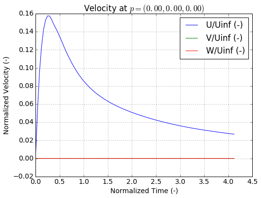
The velocity for any given probe can be plotted quickly by calling
plot_probe_data_by_id().
In [38]:
fig, ax = run.probes.plot_probe_data_by_id(0,timestep=False)
Accessing the input namelist
The input file namelist can be accessed using the namelist instance
attribute.
In [39]:
run.input.namelist
Out[39]:
OrderedDict([('configinputs',
              OrderedDict([('gpflag', 0),
                           ('nr', 5),
                           ('nti', 20),
                           ('iut', 1),
                           ('convrg', -1),
                           ('ifc', 0),
                           ('nric', 9),
                           ('ntif', 30),
                           ('iutf', 1),
                           ('convrgf', 0.0001),
                           ('ixterm', 0),
                           ('xstop', 5)])),
             ('caseinputs',
              OrderedDict([('jbtitle', 'NREL 5 MW'),
                           ('rho', 0.002378),
                           ('vis', 3.739e-07),
                           ('tempr', 60.0),
                           ('slex', 0.0),
                           ('hblref', 0.0),
                           ('hag', 295.276),
                           ('rpm', 12.1),
                           ('ut', 7.55),
                           ('geomfilepath', './NREL-5MW.geom'),
                           ('nsect', 8),
                           ('afdpath',
                            ['./airfoils/Cylinder1.dat',
                             './airfoils/Cylinder2.dat',
                             './airfoils/DU40_A17.dat',
                             './airfoils/DU35_A17.dat',
                             './airfoils/DU30_A17.dat',
                             './airfoils/DU25_A17.dat',
                             './airfoils/DU21_A17.dat',
                             './airfoils/NACA64_A17.dat'])])),
             ('configoutputs',
              OrderedDict([('diagoutflag', 1),
                           ('output_elflag', 1),
                           ('wakeelementoutflag', 1),
                           ('wakegridoutflag', 1),
                           ('probeflag', 1),
                           ('probespecpath', './probes.dat')]))])
This namelist can easily be modified and rewritten as a separate file (perhaps facilitating parametric studies of parameters).
In [40]:
run.input.namelist['configinputs']['nti'] = 30
In [41]:
import StringIO

output = StringIO.StringIO()
run.input.namelist.write(output)
In [42]:
print output.getvalue()
&configinputs
    gpflag = 0
    nr = 5
    nti = 30
    iut = 1
    convrg = -1
    ifc = 0
    nric = 9
    ntif = 30
    iutf = 1
    convrgf = 0.0001
    ixterm = 0
    xstop = 5
/

&caseinputs
    jbtitle = 'NREL 5 MW'
    rho = 0.002378
    vis = 3.739e-07
    tempr = 60.0
    slex = 0.0
    hblref = 0.0
    hag = 295.276
    rpm = 12.1
    ut = 7.55
    geomfilepath = './NREL-5MW.geom'
    nsect = 8
    afdpath = './airfoils/Cylinder1.dat', './airfoils/Cylinder2.dat', './airfoils/DU40_A17.dat',
              './airfoils/DU35_A17.dat', './airfoils/DU30_A17.dat', './airfoils/DU25_A17.dat',
              './airfoils/DU21_A17.dat', './airfoils/NACA64_A17.dat'
/

&configoutputs
    diagoutflag = 1
    output_elflag = 1
    wakeelementoutflag = 1
    wakegridoutflag = 1
    probeflag = 1
    probespecpath = './probes.dat'
/